Introduction

This post is a follow up discussion of an earlier work about recommender systems for the Santander dataset using a hybrid model combining the stacked denoising autoencoder (SDAE) with matrix factorization (MF) algorithm. I will focus on how to use the model to interpret the patterns of the dataset.

What Can We Get from the Dataset

The key information extracted from the dataset is the rating matrix and the side information of clients. The size of the rating matrix is (client number) $\times$ (product number). Each matrix element $r_{ij}$ is the total number of months that the client $i$ has used the product $j$ from 2015-01-28 to 2016-03-28. The record from 2016-03-28 to 2016-05-28 is reserved for the validation and testing process. Note that we can build a recommender system only using the rating matrix by collaborative filtering (specifcally, MF algorithm).

Besides, the client information is extracted to enhance the performance of MF, especially for the new clients without any purchase history. Both categorical (gender, nationality, etc.) and numerical (age, income, etc.) variables exist in the dataset. The categorical variables are represented by one-hot encodings, and the numerical variables can be binned and become categorical variables. These encodings are concatenated into a binary 314-dimensional vector as the input of SDAE.

The goal of the recommender system is using the client information and the purchase record from 2015-01-28 to 2016-03-28 to predict the products that are likely to be purchased in the following month.

Model Description

The figure below shows the hybrid model combining SDAE with MF. Here (Wang et al. (2015)) is a good article on this model.

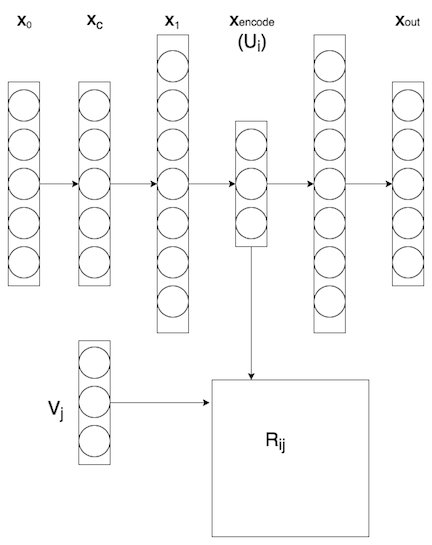
The structure of a typical SDAE is shown in the upper part of the figure above. The 314-dimensional binary encoding $X_0$ in the input layer is followed by a corruption layer $X_c$, where a Gaussian noise is added. Tied weight is applied in the SDAE, such that the SDAE has a symmetric structure. The $X_{encode}$ layer with the least number of hidden units is the encoding of the user information and will be fed into the MF algorithm.

In the MF algorithm, we need to handle the rating matrix $r_{ij}$ containing the user behavior history, which are implicit feedbacks. This is different from the explicit feedbacks such as the ratings in Amazon and Netflix, as discussed in Hu et al. (2008).

For implicit feed backs, we can construct preference matrix $p_{ij}$ and confidence matrix $c_{ij}$ according to the rating matrix. If a customer has used a certain service before, then that costomer shows preference to this service. Accordingly, the definition of preference $p_{ij}$ is given by \begin{equation} p_{ij}=\begin{cases} 1 & \text{if }r_{ij}>0\\ 0 & \text{otherwise} \end{cases}\;. \end{equation} On the other hand, we are not completely sure about the preference. Therefore, we need to define the confidence \begin{equation} c_{ij}=1+\alpha r_{ij}\;, \end{equation} where $\alpha$ describes how the confidence grows with the number of months of using the service $j$.

The MF algorithm for implicit feed back is applied in the following way. We define user matrix $U_{i,:}$ and item matrix $V_{j,:}$, where each row, written as $\mathbf{u}_i$ and $\mathbf{v}_j$, is the vector in the latent factor representation for each customer and service, respectively. We predict the preference $p_{ij}$ by $\mathbf{u}_i\cdot\mathbf{v}_j$. The preferences with different levels of confidence are not treated equally in the loss function, which is given by: \begin{equation} l=\sum_{i,j}c_{ij}(p_{ij}-\mathbf{u}_i\cdot\mathbf{v}_j)^2+\lambda(\sum_i|\mathbf{u}_i|^2+\sum_j|\mathbf{v}_j|^2)\;. \end{equation} From a probability point of view, the confidence $c_{ij}$ measures the standard deviation of the prediction to the preference.

The update rule is given by setting the derivatives of the loss function with respect to $\mathbf{u}_i$ and $\mathbf{v}_j$ to zero. Details can be found in Hu et al. (2008). Note that this article also provides a trick to speed up the training process using the sparsity of the preference matrix. In my implementation, this trick speeds up the MF algorithm by over 500 times.

Each time after the $U$ and $V$ matrices are updated, we also update the parameters in the SDAE using gradient decent, such that collaborate filtering not only receive the prediction from the SDAE, but it also provide feedbacks to the SDAE.

In the prediction process, we use the percentile ranking of the “new services” (services that haven’t been purchased by each user between 2015-01-28 and 2016-03-28 but purchased by this user in 2016-04-28) to evaluate the performace of the model. The percentile ranking is assigned according to the value of predicted preference matrix $\mathbf{u}_i\cdot\mathbf{v}_j$. A ranking of $100\%$ means the item is predicted to be the least favorable for user $i$, while $0\%$ means the item is the most favorable. A random guess should give a ranking of $50\%$, the lower the better. For new users whose purchase history is not available, we can generate the user matrix using the SDAE, thus the cold-start problem in collaborative filtering can be levitated.

Some Visualizations

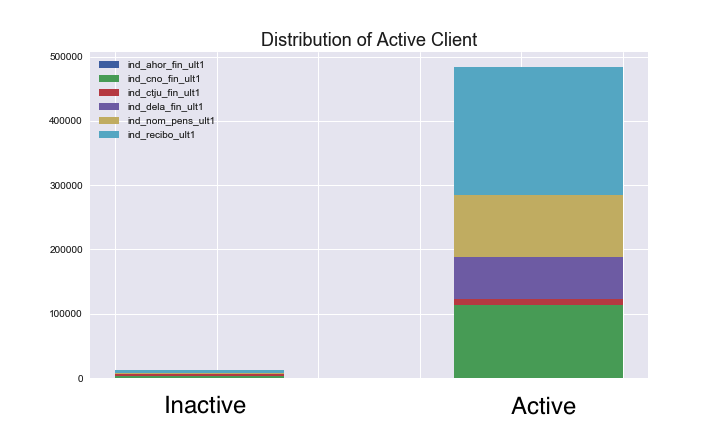
Before running the model, let’s get some insight about the dataset by visualizing the distributions of some features. The following graph shows the distribution of the activate/inactive clients for some products. It is not surprising to see that most customers that have chosen any products are active clients. If we see a new client whose state is “inactive”, it is reasonable to assume that this client will not use any new service.

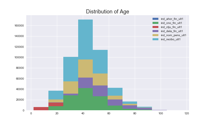
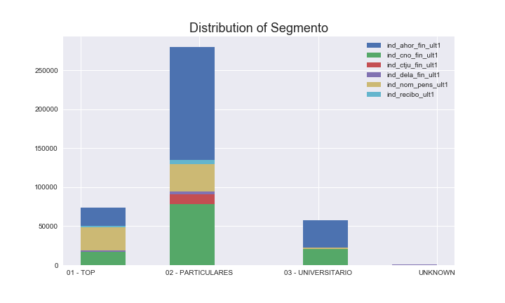
The following graph shows the distribution of age and segmento (the level of clients) for different clients. Unlike the feature for activate/inactive clients, different product shows quiet different distributions. For example, the Junior Account (nd_ctju_fin_ult1) is mainly used by clients below 20 years old; the people over 80 years old are less likely to take risk and prefers long-term deposits (ind_dela_fin_ult1) than other services. In addition, the clients in the top level are more likely to use the pension service rather than saving account compared to the clients in the lower levels. Such difference between products implies that the user information can be very helpful when predicting the customer behavior.

Results and Interpretation

I applied a strong $l_2$ regularization for the user and product matrix ($\lambda=400$). For the users with purchase history, the percentile-ranking is $9.42\%$. For the new users with no purchase history, I first calculate the user matrix from the SDAE, and calculate $\mathbf{u}_i\cdot\mathbf{v}_j$. The percentile-ranking for these new users is $10.33\%$. In comparison, if we don’t have the SDAE and predict the purchase behavior by a random user matrix, the percentile-ranking is over $20\%$. That means the SDAE is learning useful information for making the prediction.

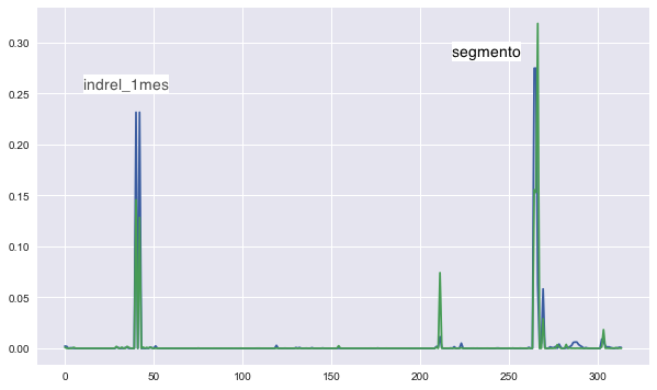
Let’s try to understand what is learnt by the SDAE. The green line in the figure above shows the absolute value of the weights for one of the hidden units. There are two sharp peaks at the “segmento” and “indrel_1mes (customer type)” feature, meaning SDAE regards these two as the most important features. Similarly, the country of residence and age are also important features. The weights for other hidden units have similar peak positions, while the strength of each peak varies. Note that most features have negligible weights, meaning they are regarded as unimportant by the model. This is a consequence of applying $l_1$ regularizations to the weights.

I also plotted the Fisher score for each of the binary encodings in $X_0$ for the user information in a blue line in the figure above. The Fisher score describes how well can each feature separates the data points from different categories while keeping the data points in the same category clustered. For each feature, the Fisher score is given by \begin{equation} F(X_0^j)=\frac{\sum_{k=1}^c n_k(\mu_k-\mu)^2}{\sigma_k^2}\;, \end{equation} where $k$ in the numerator is summed over all categories; $\mu_k$, $\sigma_k$ are the mean and standard deviation of the feature $X_0^j$ in each category, $\mu$ is the mean of all data points, and $n_k$ is the number of data points in category $k$. More details of the Fisher score can be found in this article. Now we concentrate on how well the features separate the clients that have used the service “ind_recibo_ult1” from those who haven’t. The curve for the Fisher score strongly overlap with the distribution of weights, meaning the SDAE is trying to find out which features can do the best to separate the clients with different preferences. If we calculate the fisher score based on other services, some addition peaks can appear, while the most prominent ones are still “segmento” and “indrel_1mes”.

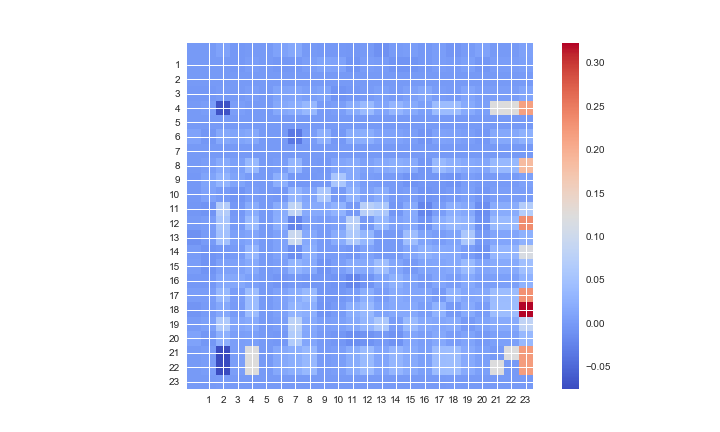
Furthermore, we can get additional insights from the MF algorithm. The paper by Hu et al. (2008) proposed the following way to explain the model. Simple mathematical derivation shows that the preference matrix can be written as \begin{equation} p_{ui}=\sum_j s^u_{ij}c_{uj}\;, \end{equation} where $s^u_{ij}=v_i^T(V^TC^uV+\lambda I)^{-1}v_j$, and $C^u=Diag(c_{u:})$. The (number of products $\times$ number of products) matrix $s^u_{ij}c_{uj}$ represents the influence of the purchase history of $j$ on the decision of customer $u$ to purchase the item $i$. The following figure plots the matrix $s^u_{ij}c_{uj}$ for one of the clients. This client started to use the e-account (‘ind_ecue_fin_ult1’, labeled by 12 in the plot) in 2016-04-28, which is a new service for this client. On the row labeled by 12, the strongest contribution comes from the 23rd column representing the direct debit service. Indeed, this client has used the direct debit service for 8 months, and he/she now wants to make it electronic. We can do a similar analysis each time a client start to use a new service and find out the purchase history that has the most important influence on the new purchase.

Summary

In sum, the hybrid model that combines SDAE and MF not only gives rise to good predictions to the customer purchase behavior, but also provides insights to the reason of these purchases. It is necessary to realize that this model has used some assumptions that has not been explicitly pointed out. For example, when constructing the rating matrix, the purchase history from 2015-01-28 to 2016-03-28 are aggregated together. Therefore, what the model receives is an average effect in the two-year-long time slot. By using this averaged data to predict the purchase in 2016-04-28, we need to make the assumption that the preference of clients does not depend on the month of the year. However, this is not exactly true. In this discussion on Kaggle, someone observed that the purchase in June can be very different from other months. Training only on the data in June 2015 can give a pretty good prediction for June-2016. On one hand, this is a concrete evidence for the importance of feature engineering and the insight of the problem. On the other hand, in a more general sense, time-dependent models for recommender system deserve more study in the future. Here is a good survey on this topic.